Unquantifiable Error in Graphene Stiffness

Most Graphene Measurements are Wrong

Diamonds in the Plane

"What the fuck is graphene?" asked the barback in between shots of Rumple Minze. Well, I responded, it's like if a diamond was a thin sheet. "What does that mean?" Diamonds are really hard, right? That's why people use them for jewelry and such. "I guess." They're really hard because of how the diamond atoms --- carbon atoms --- are bonded together. With graphene, you have those really strong atomic bonds, but they all lie in a flat plane. Those bonds mean that graphene has a lot of very, very desirable properties like extraordinary strength and conductivity.

"So does this stuff cost as much as a diamond?" Nope. Not even close. "So it’s like really expensive?" Um... So... In bulk, graphene is called graphite. It's the same stuff they put in pencils. "Oh..." Yea... But it's got some pretty incredible properties!

The molecular structure of a three-dimensional diamond (top)[1] and a two-dimensional "diamond" known as graphene (bottom)[2]. The dots are carbon atoms. The cylinders linking the dots are covalent bonds. The images are not at the same scale.

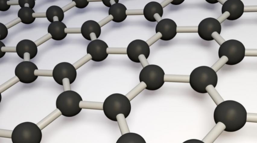
"So what do you do with it again?" In my group, we try and use graphene to make stronger materials. I'm the guy who measures those new materials to see if they're any stronger than the old materials.

For instance, the army wants stronger tanks. The oil drillers want stronger bits. Boeing wants a stronger, lighter airframe. So they collectively throw, you know, tens of millions of dollars at graphene research. "That sounds cool." I mean, I don't see that kind of money. I'm just a grad student.

And... I'm not entirely on the graphene bandwagon, either. I mean, graphene definitely has some pretty great properties. But I think a bunch of people have been incorrectly measuring it to be stronger than it actually is. And that's a bit of a problem considering that big pile of cash being thrown at the field.

Atomic Force Microscopy - An Introduction

Since a single layer of graphene is so thin, the material is often measured with an atomic force microscope. The best explanation of this technique involves a butter knife. If you don't have a butter knife, you can use your forearm. Hold the knife (or forearm) horizontally with the flat part parallel to the table. Now imagine a very, very sharp point protruding downward from the end of the butter knife and just barely touching the magazine open in front of you. Move the butter knife with its imaginary sharp point back and forth over the text of the magazine as if you were reading the magazine, magically, through the tip and butter knife.

That's how an atomic force microscope (AFM) works. An AFM, one of the greatest scientific inventions of the past 50 years, is effectively a butter knife, with a very sharp tip. Of course, the microscope uses a very small butter knife, and the sharpness of the tip is barely conceivable to even seasoned microscopists. (Seriously. From time to time, I still catch myself squinting at a tip as if all I needed to do was squint harder to see something 100x smaller than the resolving power of optical microscopes.) But at the end of the day, it's that simple. Butter knife. Sharp tip. That's it.

Abe doing the science. Because AFM cantilevers (butter knives) are so small, they are attached to larger chips so that humans can handle them. The AFM chip is the black rectangular object that Abe is looking at. If you look closely, you can see the AFM cantilever (our butter knife) extending vertically upward from the top of the chip. The sharp tip is a mere speck (at these length scales) at the very end of the cantilever.

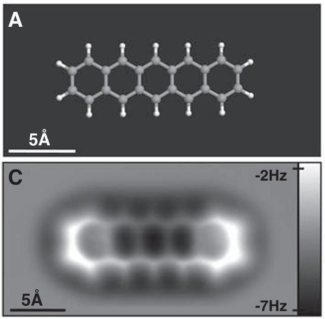
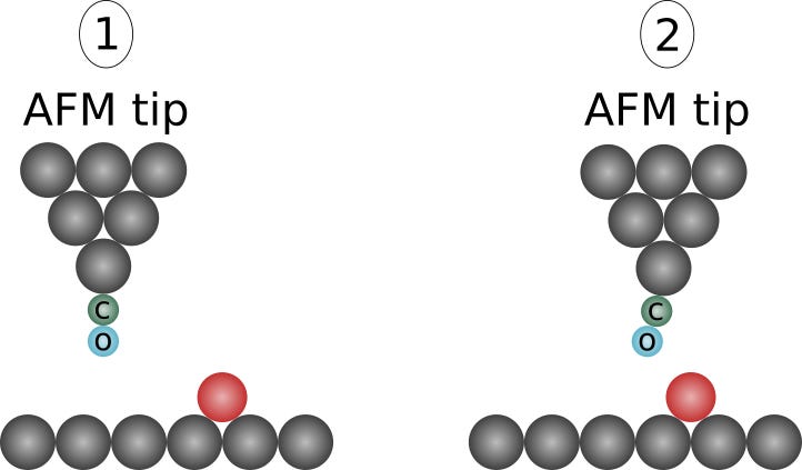
So what can a butter knife with a sharp tip do for capital-S Science? A lot, it turns out. The coolest (literally) AFM experiments involve using a tip that's only a few atoms wide, attaching a single carbon monoxide (CO) molecule to the end of the tip and then imaging at near absolute zero temperatures (5 Kelvin, -270 Celsius, -450 Fahrenheit) so that the carbon monoxide doesn't rotate side to side. (The carbon monoxide-tip connection can be thought of as a ball-socket joint. The low temperatures reduce measurement noise by reducing the Brownian motion of the system.) With this setup, you can measure individual covalent bonds (~0.15 nanometers long). Pretty cool.

A ball and stick model of pentacene (top) and a sub-atomic resolution AFM image of pentacene (bottom)[3].

An AFM Tip with a carbon monoxide molecule attached to the end. The carbon monoxide is particularly prone to rotation (right image) requiring very low imaging temperatures[4].

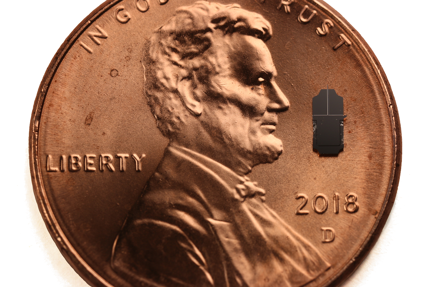
You don't need to measure at sub-nanometer length scales to contribute to capital-S Science. There are a number of other things --- agglomerations of atoms --- that are difficult to image at a 10-nanometer resolution (100x larger than the subatomic experiment above). Most high resolution imagery is collected using electron microscopes, which generate images by shooting electrons through materials (transmission electron microscopes, TEMs) or by bouncing electrons off materials (scanning electron microscopes, SEMs). If shooting electrons through a material would damage or distort the material (soft materials, cells, polymers) or if electrons don't bounce off the material but instead stick to its surface (non-conductive materials), then it can be really challenging to get high-resolution images with electron-based techniques. These sorts of materials --- soft, polymeric, cellular, non-conductive --- are where the atomic force microscope really shines.

A single strand of DNA imaged with an atomic force microscope[5] Note the visible double helix, the ridges along the DNA strand. The white arrows indicate the slow-scan imaging direction. The colorization corresponds to height.

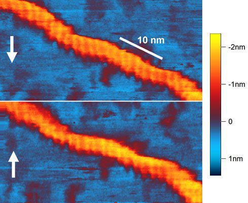
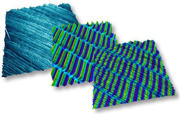
Since the AFM creates its images using a sharp tip, surface conductivity does not affect imaging. Since AFM images are constructed from the motion of a physical probe, we can use the probe to measure other properties of our atomic agglomerations. If we apply a voltage to the tip, we can measure minute changes in surface conductivity or magnetism. If we wiggle the butter knife at different frequencies, we can measure minute changes in stiffness.

I spent 7 years of my PhD doing just that - trying to measure, as accurately as possible, nanometer-scale differences in the surface stiffness of tire rubbers. What? Tire rubber? That black kind-of-squishy stuff that sets me back $700 every few years? I honestly thought the same thing when the project was proposed. However, if you zoom in far enough (below about 1000 nanometers), tire rubber is an incredibly complicated and interesting material. But I digress. This post is not about tire rubber. This post is about making very accurate graphene measurements using the atomic force microscope.

AFM images of a hard disk drive[6]. Each square measures 20 x 20 micrometers. Topography (left), magnetic force (center), and magnetic force overlaid on three-dimensional topography (right).

On Publishing

So why are you writing a blog post? Didn't you get to sling all your academic jargon into a three-hundred-page dissertation? Aren't you supposed to publish in paywalled journals? To the first point, my dissertation omitted these findings, arguably my most significant research contribution. Like all good science, this work was discouraged and then rejected by esteemed members of the academy. To the second point, despite the 9-year duration of my postgraduate odyssey, I only went to two conferences and generated zero publications. To the third point, Adam Mastroianni makes an excellent case for the abolition of peer review.

Such little academic "output" is highly unusual. It may seem a little odd to outsiders, but papers are the currency of academia. The more papers you publish, the more status tokens you accrue. If you accrue enough status tokens, the university agrees not to fire you. (This is called "tenure".) If you accumulate even more status tokens, you get to list some rich frat bro's name after your name on emails. (These are called "endowed professorships".) (And what am I trying to do with this piece other than gain status tokens?) I generated zero papers. I have zero status tokens. I was effectively dishonorably discharged with a degree.

Aside: But isn't publishing how we generate New Knowledge and share it with the world!? Technically, yes, but the quality of most academic research is quite poor. Most of it can't be reproduced. And most of what is generated is locked behind paywalls. The primary motivation to publish for most academics seems to be status. As such, I'd argue that "status token" is a more apt characterization of most peer-reviewed manuscripts. (The word "most" is doing a bit of work here. There are honest professors and honest researchers. However, the academic incentive structure does not do a great job of rewarding honest research.)

Not a butter knife. The author's model cantilever constructed from a flimsy 30-year-old ruler, a piece of window-blind hardware, and scotch tape. Shown with a penny for scale.

Infinite, Unquantifiable Measurement Error

There are a few thousand peer-reviewed publications each and every year reporting very accurate and very precise measurements collected using an atomic force microscope. My primary finding, from 7 years of hard labor, was that the vast majority of these papers reported measurements with unquantifiable error. Not only are the vast majority of these measurements inaccurate, they are inaccurate by an unknown amount. Further, it can be shown that, in some cases, the error can be infinite. (I will provide such an example below.)

To put this finding in context, most academics believe the field of atomic force microscopy is pretty well established. Again, there are thousands of papers each year reporting quantitative AFM measurements. The general consensus has been that these problems have been solved. My preliminary examination committee did not believe that such an error could exist. Further, they asked me to omit these findings from my dissertation.

Errors in atomic force measurements matter because a material can be deemed the "strongest material" based on AFM measurements alone. A lot of people (aerospace, defense, oil exploration) are interested in finding stronger and stronger materials. These people will invest a lot of money into the research and development of a material if it shows promise.

In the mid 2000s, AFM measurements showed graphene and carbon nanotubes to be some of the strongest materials in the world[7]. (Fun fact: As an undergraduate, I was a member of the racecar club whose shop abutted the room that contained this particular AFM.) Subsequently, millions of dollars were poured into the development of graphene-enhanced materials. In the process, many, many more AFM measurements were made showing how materials could be made stronger, for example, by adding a layer of graphene on the surface.

I do not doubt that graphene and carbon nanotubes are very strong materials. Their covalent lattice generates bond strengths similar to those in diamond. I will claim, however, that AFM measurement errors --- specifically the one discussed below --- can make these materials appear much stiffer than they actually are, sometimes infinitely stiffer.

The good news is that the findings that I'll present here have been vindicated. I did this particular bit of research in the early months of 2019. At the end of 2020, my preliminary examination committee rejected this work. In the early months of 2021, flustered by my rejection, I reached out to Asylum Research, the leading AFM manufacturer. They subsequently asked me to interview for an R&D role. (They didn't hire me due to the lack of status tokens.) A few weeks ago, Asylum Research released a new atomic force microscope which has the ability to correct the measurement errors that I discovered and will present below. This post is the first time that I'm publicly discussing this work. (I have no financial ties to Asylum Research and do not stand to benefit financially from the sale of their microscope.)

Reading the Cantilever - AFM Measurement Generation

To understand how error can enter a measurement, we need to understand, in detail, how the measurement is generated. We need to dig down to the very core of the microscope's operation. Unfortunately, each level of depth adds a bit of complexity. From here on out, descriptions will get a bit technical, but I will try to keep things as simple as possible. After all, we are talking about a butter knife with a sharp tip.

A sketch depicting the core components of an atomic force microscope. The functionality of these components is described below.

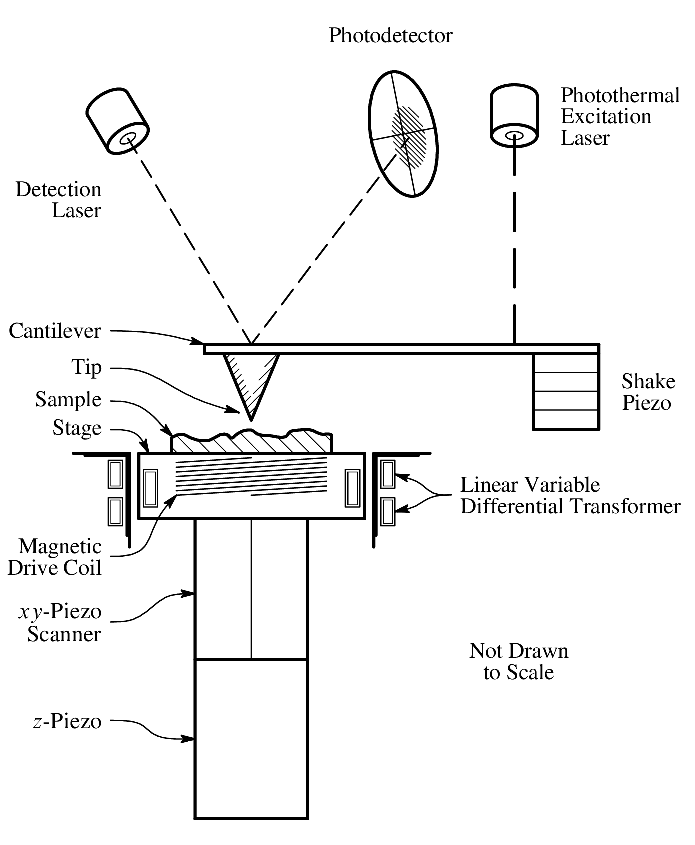
The heart of an atomic force microscope is a sharp tip, often with a radius of 10 nm or less, affixed to the end of a cantilever of micrometer dimension.

During “tapping mode” imaging, the cantilever is oscillated near its fundamental resonant frequency by one of three forcing methods: a shake piezo at its base, a photothermal excitation laser focused near its base (preferred), or by an electromagnetic coil at the tip.

To create an image, the tip is raster scanned over the sample surface. (This is just like reading a book - back and forth, line by line.) A detection laser, reflected off the free end of the cantilever and onto a photodetector, generates an electrical signal proportional to the tip’s angular deflection.

A controller adjusts the tip–sample distance via the z-piezo to maintain a constant oscillation amplitude. Alternative imaging modes control the tip–sample distance using different parameters such as a frequency shift or the quasi-static cantilever deflection.

A linear variable differential transformer (LVDT) measures the sample stage’s z-position, supplying the voltage signal used for sample topography or height.

Two voltage signals are recorded while imaging. The photodetector signal is proportional to the cantilever’s angular deflection, and the LVDT signal corresponds to the vertical position of the sample stage. Put simply, the challenge of AFM quantification is accurately converting these two voltages to material properties of the sample (conductivity, stiffness, etc.).

Additional sensors and calibrations are required to measure the x- and y-position of the cantilever's base relative to the sample. We will not discuss this lateral measurement system as it is not relevant to our analysis. For our purposes, the cantilever's base and the sample can be considered to be fixed in x and y. We will discuss, in detail, how the cantilever deforms as it is extended toward the sample and retracted away from the sample.

LVDT Calibration

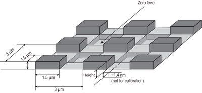
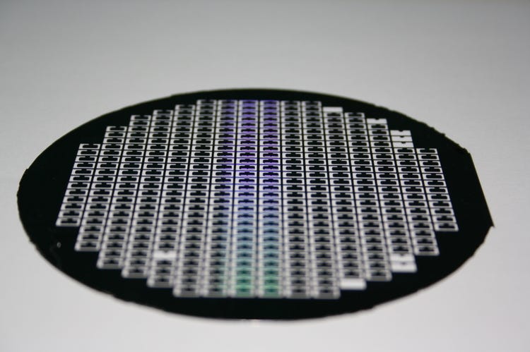
Of the two voltage calibrations, the LVDT calibration is (1) straightforward and (2) stable. The LVDT voltage is calibrated by imaging a grid geometry with a precise and accurate height. After imaging the grid, a LVDT-voltage-to-height calibration parameter is computed. The LVDT sensor system is quite stable over extended periods of time and does not depend on one's choice of cantilever.

A sketch of a commercially available AFM test grating for x, y, and z (LVDT) calibration[8].

Aside: One of the biggest advances in atomic force microscopy was the LVDT that Asylum Research developed for their Cypher AFM[9][10]. Their LVDT is an ingenious reimagination of a typical LVDT and is incredibly precise and stable. Their LVDT is a pretty remarkable technological achievement that is often overlooked by the academic AFM community.

Each Butter Knife is Unique

Cantilever calibration is a bit of a rat's nest compared to LVDT calibration.

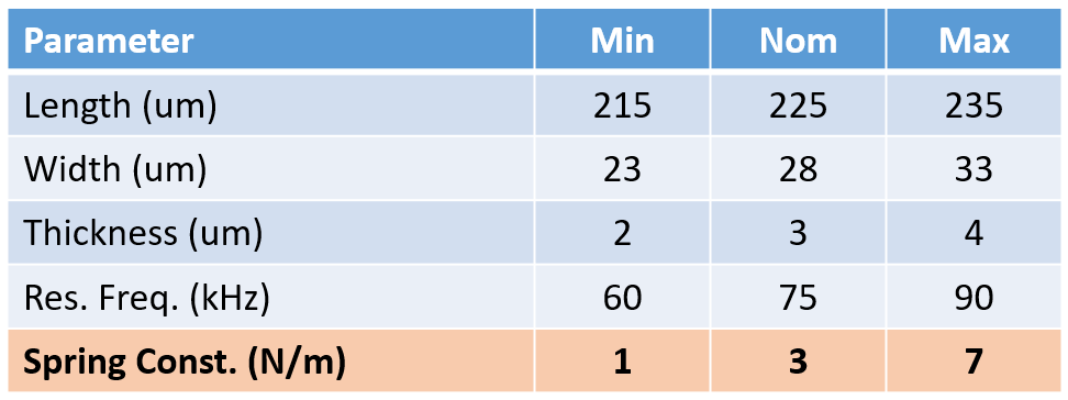
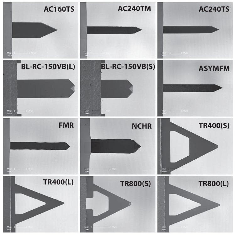
Why do we need to calibrate cantilevers? Because every single cantilever is unique. AFM cantilevers come in an incredibly wide variety of sizes and shapes optimized for different sample materials. For example, biological cells are very soft. Crystals are very hard. Both materials can be imaged with an AFM. Optimal imaging of biological tissue requires a very different cantilever and imaging conditions than sapphire crystals.

Although cantilevers can be made from most any material, most cantilevers are manufactured from single crystal silicon wafers similar to those used to make integrated circuits and GPUs. Due to the stochastic nature of the silicon etching processes used to remove material and create the cantilever, two cantilevers from the same wafer can vary by an order of magnitude in stiffness, sensitivity, and spatial resolution.

Typical dimensional and parameter ranges for the BudgetSensors Multi75GD-G cantilever. The spring constant can vary by an order of magnitude.

AFM chips still attached to a silicon wafer during fabrication[11].

AFM cantilevers (butter knives) in many different shapes and sizes[12]. Scale bars range from 20 to 50 micrometers.

A Simplified Calibration

If we simplify cantilever calibration as much as possible, we are left with two required measurements: (1) a force curve to determine the cantilever's sensitivity and (2) a thermal (Brownian) vibration measurement to determine the cantilever's spring constant. With these two calibrations, we can determine the applied force and indentation distance at the tip. If we then throw in a tip size and shape approximation, we can obtain the mechanical response (stiffness) of a material at some pretty incredible resolutions.

Aside: The cantilever tip's size and shape are also very important parameters in all indentation models. We currently do not have a particularly good way of calibrating very sharp (< 100 nanometer) tips. Further complicating matters, tips wear and change shape during imaging[13].

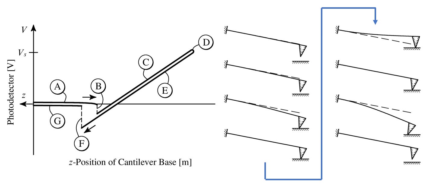
During a force curve, the cantilever's base is extended toward and then retracted away from a sample's surface. (The free end of the cantilever deflects in response to forces acting on the tip.) During extension and retraction, the tip makes and breaks contact with the sample surface. The slope of the contact region, in a plot of the photodetector voltage versus the z-position of the cantilever base, is then used to calibrate the photodetector voltage to a vertical cantilever deflection distance. To ensure only the cantilever is deflecting during calibration, a very hard substrate (such as single crystal sapphire) is used for this measurement. (In a few paragraphs, we'll take a deep dive into each feature of the force curve.)

An ideal, quasi-static force curve (left) and corresponding cantilever deformation (right). The tip begins its journey far removed from the influences of the sample surface. As the tip approaches the sample (A), long-range surface forces pull the tip and sample towards one another. This attraction often results in visible deflection of the cantilever before snap-on. Eventually, the attractive forces overwhelm the elastic resistance of the cantilever, and the tip jumps into contact with the surface (B). As the base of the cantilever continues to move towards the surface, sample elasticity resists further intrusion by the tip, compelling the cantilever to deflect upward (C). Eventually, the approach stops (D). The cantilever base is then raised or retracted from the sample surface. Less deflection is required of the cantilever, and less force is exerted between the tip and sample (E). The pull of the cantilever eventually overcomes the attractive influence of the sample and the cantilever snaps upward and away from the sample (F). Retraction continues until the cantilever base reaches its starting position (G). The contact regions (C) and (E) are the portions of the curve that are of mechanical interest.

With the voltage-distance calibration in hand, a fast-Fourier transform of the cantilever's thermal response is collected. Using the magic of statistical physics and the Equipartition Theorem, the cantilever's spring constant can be obtained. This is a surprisingly accurate measurement, whose theory deserves a thorough explanation in its own post.

Note that the model commonly used to fit the first resonant peak of the thermal response appears to have a mathematical error[14]. I believe the relation provided in footnote 39, without an accompanying derivation, is missing a factor of 2. I rederived this expression and validated my spring constants using finite-element analysis (FEA). Both the rederivation and the FEA analysis supported my claim of a missing factor of 2. (This is why you always check the math in the paper and double check your own math.)

The thermal response of an AFM cantilever. The first three resonant peaks are visible and are labeled on the horizontal axis.

A fit of the first resonant peak.

Beam Theory as Glue

The astute dynamicist will note that the quasi-statically deflected beam in our force curve has a slightly different normalized shape than a beam oscillating at its first resonant frequency. The astute dynamicist will also note that the elastic energy of the normalized beam shape is proportional to the spring constant of the shape. Therefore a quasi-static deflection will have a slightly different spring constant than a first resonant mode oscillation. (This math can readily be found in textbooks covering beam dynamics.)

Why does this matter? Well, I oversimplified things a moment ago. The photodetector isn't actually measuring vertical displacement at the end of the cantilever. The photodetector signal is actually proportional to the angle of the deflected free end of the cantilever. This is a critical difference.

The force curve described above quasi-statically deflected the cantilever. Our thermal calibration measured the vibrations of the cantilever's first resonant frequency. To use the quasi-static sensitivity calibration for our thermal (oscillatory) measurements, we need to adjust the sensitivity to account for the different beam shapes.

Normalized mode shapes for the quasi-static, first, second, and third modes for a rectangular cantilever. The frequency ratios are with respect to the resonant frequency of each mode. The angle ratios compare end-of-cantilever angles.

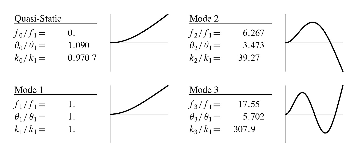
Converting between quasi-static and oscillatory measurements is fairly straight-forward. In some AFM software, this conversion parameter is called the "kappa factor". Since larger cantilever angles will produce a larger photodetector signal, we simply need to adjust for the difference in angle at the ends of the normalized quasi-static beam θ0 and the normalized first resonant mode shape θ1.

Now, the academic AFM community would say that we have everything that we need to run a "quantitative" AFM experiment. We have the vertical displacements of the sample (via LVDT) and the cantilever tip (via the photodetector). We have the applied force at the cantilever tip. And we have an approximation for the tip size and shape. We're ready to take some measurements!

Validating our use of Beam Theory

Before we get ahead of ourselves and start collecting data, let's first validate the use of elastic beam theory to convert between quasi-static and oscillatory calibrations.

In our sensitivity calibration example, we used a quasi-static force curve. It is also possible to collect a force curve while oscillating the cantilever at its first resonant frequency. During an oscillatory force curve, the oscillation amplitude decreases as the cantilever approaches the surface. During each reduced-amplitude oscillation, the tip strikes the sample surface. The amplitude is reduced simply because there is less vertical space for oscillation.

Measuring the slope of the photodetector's amplitude (a voltage) versus the z-position of the cantilever's base, we can obtain a cantilever sensitivity S1 for the cantilever's first resonant mode.

An oscillatory force curve depicting the sensitivity calibration S1. A{1,0} is the amplitude of oscillation far from the sample surface. A{1,S} is the setpoint amplitude for this force curve. The nonlinearity of the tip-sample interaction causes a small hysteresis between the extension and retraction.

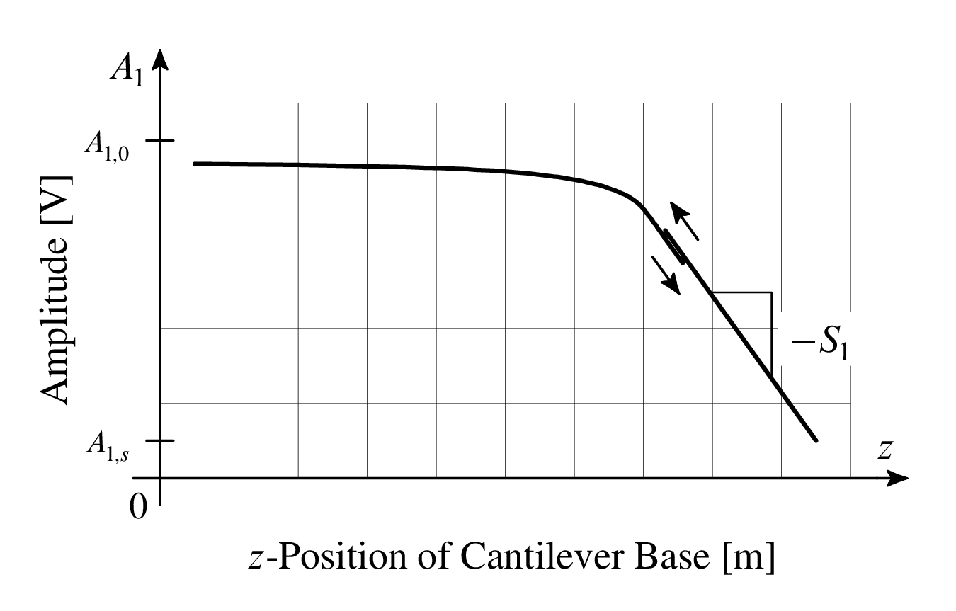
Let's denote the quasi-static sensitivity S0. Let us assign θ0 to the angle at the free end of the normalized quasi-static beam. Finally, let θ1 be the angle at the free end of the normalized first resonant mode shape. The larger angle will generate a larger photodetector voltage for the same amount of vertical deflection. If we define our sensitivity with SI units of volts per meter, then we would expect the following relationship:

\(\frac{S_0}{S_1} = \frac{\theta_0}{\theta_1}\)

We can check this expression using real sensitivity measurements taken from real force curves. Note that for the figures below we will report inverse sensitivity (1/S values) since the numbers are more human-readable.

A quasi-static sensitivity calibration force curve. The contact region for the extension segment has an inverse sensitivity 1/S0 of 45.75 nm/V. The retraction sensitivity is 43.98 nm/V. The averaged sensitivity is 44.87 nm/V.

An oscillatory sensitivity calibration force curve. The contact region for the extension segment has a sensitivity S1 of 40.73 nm/V. The retraction sensitivity is 40.83 nm/V. The averaged sensitivity is 40.78 nm/V.

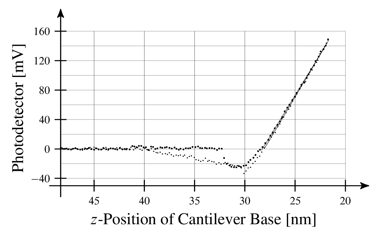
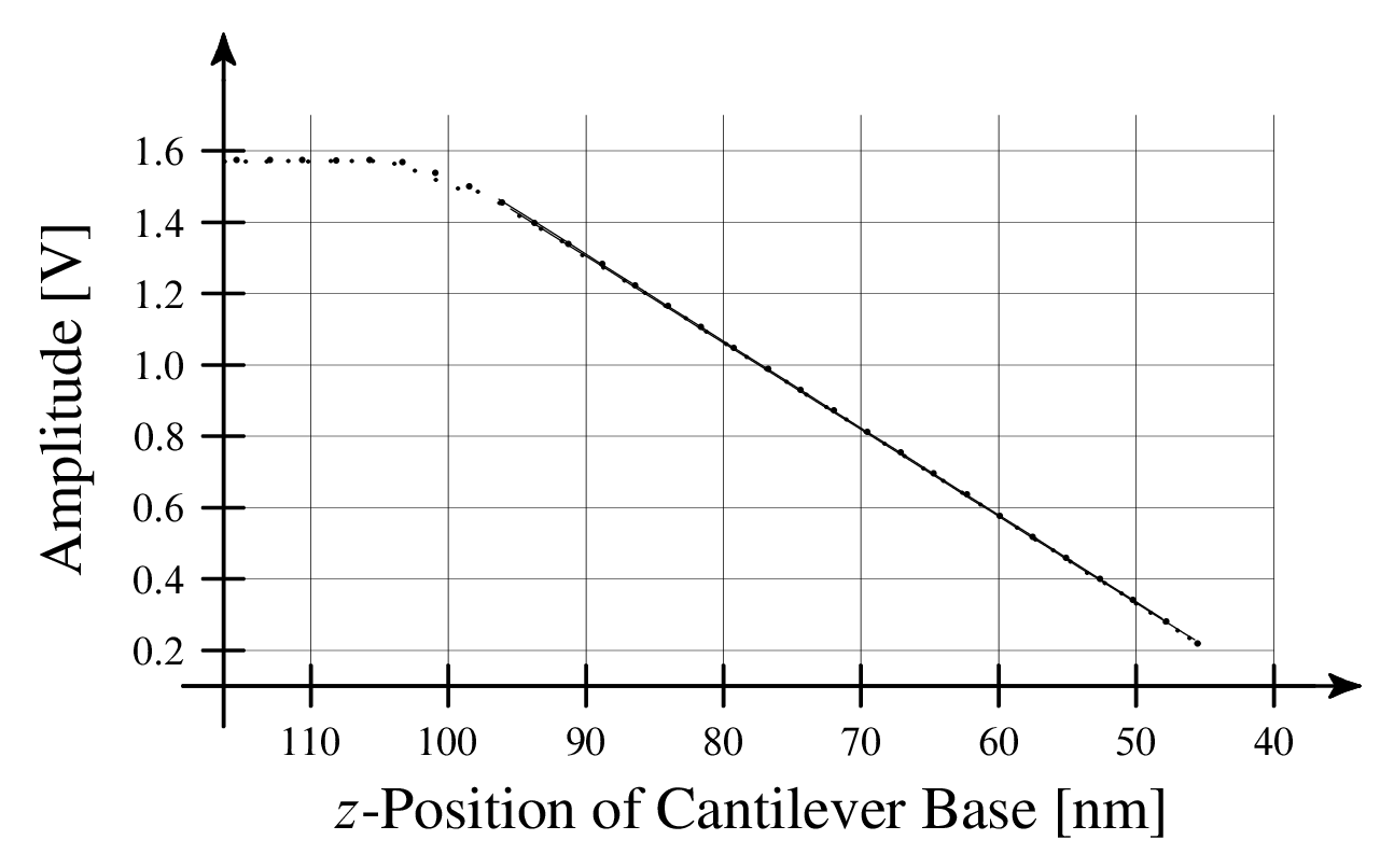
From Euler-Bernoulli beam theory for a rectangular cantilever, the expected ratio of S0 / S1 is 1.09 = θ0 / θ1 [27]. The actual ratio from these sensitivity measurements is 0.91, a difference of 17%. Considering the sensitivity and precision of the atomic force microscope, this 17% discrepancy is HUGE. If we compute a final elastic modulus (stiffness) using --- separately --- the S0 and S1 sensitivities, we obtain a 25-35% difference in the final modulus values. This amount of error can be the difference between a material being passed over for further development or registering a new material stiffness record.

A More Accurate Beam Model

One possible explanation for the 17% discrepancy is that it is not a discrepancy at all. AFM cantilevers aren't exactly rectangular. Maybe the rectangular beam approximation was an erroneous choice.

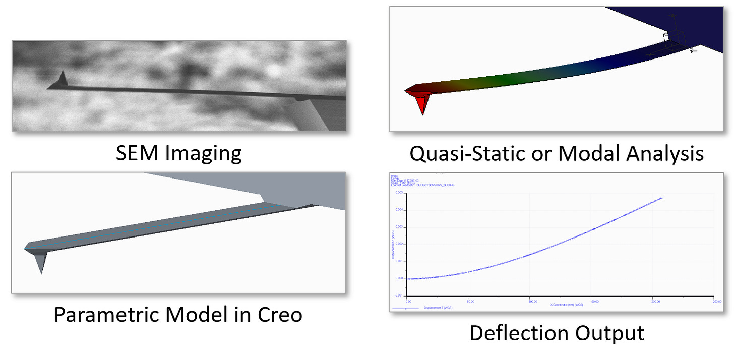
To test this idea, I asked my lab mate, Matt Robertson, to measure an AFM cantilever using the scanning electron microscope (SEM). I obtained the silicon crystal orientation and elastic modulus from the cantilever's manufacturer. I then built a very accurate model of the cantilever in Creo Parametric, a three-dimensional computer-aided design (CAD) package. Using the CAD package's modal analysis and finite-element analysis (FEA) tools, I obtained the first resonant mode shape and a quasi-statically deformed shape. Finally, I normalized the deformations and obtained the slope at the end of both cantilevers. The final end-of-cantilever angle ratio θ0 / θ1 was 1.063. Therefore, our original 1.09 was a decent approximation.

An overview of the cantilever-model generation process from SEM image, to parametric model, to finite-element analysis, to spring constant and cantilever angle analysis.

Additional Ignorance Signals

I wasn't the only one who noticed the cantilever calibration discrepancy. The AFM laboratory manager at the University of Illinois noticed it, too. So did NIST and Asylum Research. However, no explanations had been proposed. Meanwhile, thousands of papers were being published each year pushing peer-reviewed quantitative values based on questionable calibrations.

An excerpt from a post on the Asylum Research forum.

Aside: The problem with all these inaccurate measurements is that they wind up being a tremendous waste of scientific effort. For example, an experimental research group will publish a measurement and then a theoretical research group will spend a few months building a model for that measurement. The theoretical group will publish their erroneous model and it will get picked up by another group. Multiply this wasted effort over many years and hundreds of graduate students and you start to get a sense of the scale of wasted effort due to sloppy science.

At some point while I was investigating sensitivity calibration, I noticed that the extension and retraction contact regions didn't seem to overlap. In fact, they seemed to have a slightly different slope. Measuring the slope of the extension and retraction portions revealed that they did indeed differ (by 3.9% in the example below). Although this difference was not large, it was not negligible either.

I started to wonder. For sensitivity calibration, should I use the extension part of the force curve or the retraction part?

In this quasi-static force curve, the extension curve has an inverse sensitivity of 1/S0 = 45.75 nm/V. The retraction has an inverse sensitivity of 43.98 nm/V. The average of both curves is 44.87 nm/V. The extension and retraction sensitivities differ by 3.9%.

When I started investigating this question, I found three different perspectives and no clear explanation as to why one option was preferred over the others. This ambiguity signaled a genuine lack of understanding in the AFM community.

One of the AFM tomes suggested I use the extension curve "in order to exclude the influence of surface energies"[15]. My advisor said to use retraction due to fewer dissipative effects. Another source told me to use the average of extension and retraction without providing a rationale[16]. Some sources provided no guidance whatsoever[17][18].

So what causes these discrepancies? Which calibration method is the correct, if any?

Cantilever Deformation during a Force Curve

Recall that the photodetector measures the angle at the end of the cantilever. Anything that affects the angle of the cantilever's free end will affect our AFM measurements.

What might affect the angle at the end of the cantilever? How about a lateral force at the tip? A lateral force at the tip would cause a bending moment on the cantilever, which would certainly affect the measured angle at the end of the cantilever.

How likely is it that the tip would encounter a lateral force? Let's consider ideal cantilever deformation again.

A zoomed-in sketch depicting the normal Δz and lateral Δx translation of the tip during cantilever deflection.

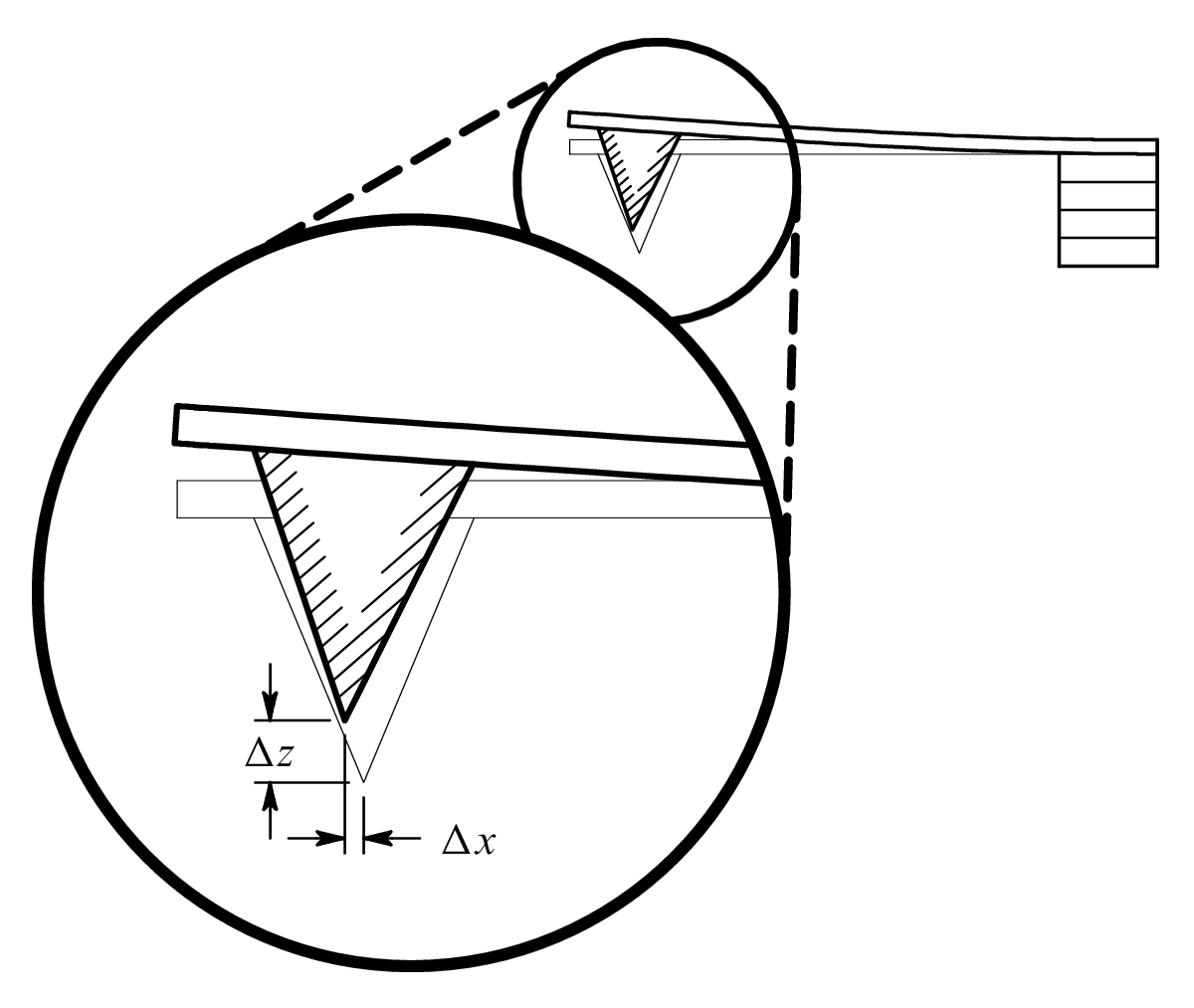
Notice that our ideal cantilever deflection actually requires a very small amount of lateral tip translation Δx. The lateral translation can amount to a single nanometer or less. However, the lateral motion is absolutely critical if we are to obtain the ideal/expected quasi-static deformation shape. The lateral translation is critical. Critical. Critical. Critical. If the lateral translation is impeded or restricted, the cantilever will deform differently and a different angle will be measured by the photodetector.

Further, as we'll describe below, there can be cases where lateral forces affect measurements but the effects are not readily detectable or measurable. An even more problematic situation can arise when the lateral forces are not detected and differ between the calibration surface and sample surface.

Observation

Let's test this lateral force hypothesis. If there are any lateral forces affecting tip deformation, then we should be able to see them as a hysteresis between the extension and retraction segments in the contact region of the force curve. Admittedly, we don't really see a hysteresis in the quasi-static force curve provided above. But what if we pressed a little harder and really forced the cantilever to slide?

An illustration of hypothetical lateral tip forces during extension and retraction.

A crude sketch of how friction might affect the extension and retraction signals. Note that the transition from extension to retraction is not illustrated as it was not fully conceptualized at the time of illustration.

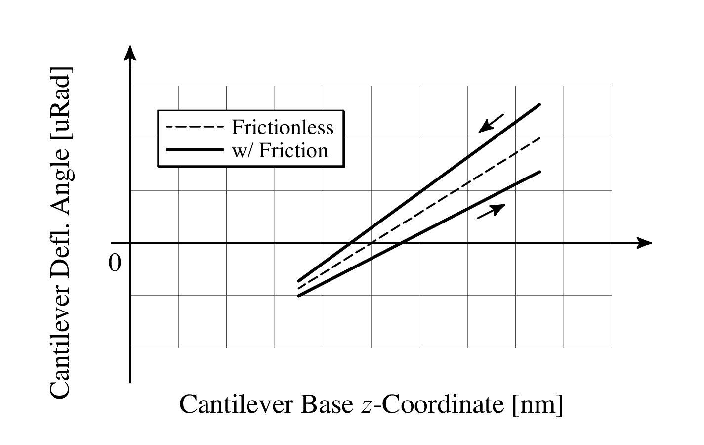
If we press hard enough, a hysteresis does appear in the force curve. We can attribute this hysteresis to frictional forces acting in different directions during extension and retraction. The hysteresis may appear small and possibly insignificant. However, small changes in the slope of the force curve can cause surprisingly dramatic variation in the computed elastic modulus of a sample, especially for very hard materials.

A sensitivity calibration force curve collected from a sapphire sample. Three segments are visible in the contact region, forming a triangular hysteresis. The extension portion is the bottom segment. The top right segment is the transition from extension to retraction. During this transition, it is believed that the tip is fixed in place. During the top left segment, the tip is presumably sliding as it is retracted.

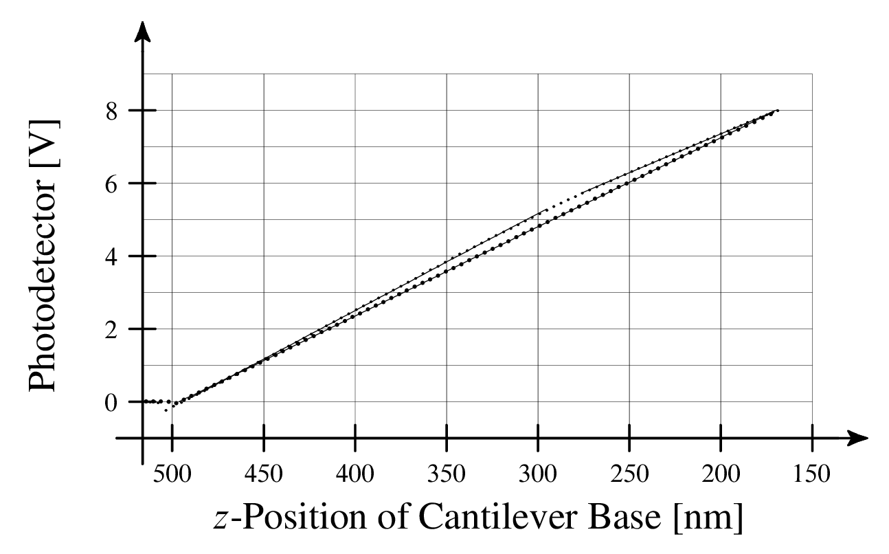
We can also simulate tip-sample friction during a force curve. To further investigate these ideas, I built a model of the cantilever-tip-sample system that include elasticity, adhesion, and tip-sample friction. Tuning model parameters to simulate a tip sliding during extension and retraction, we can obtain a force curve with the same geometry and features as our experimental force curve.

One of five images that define the cantilever-tip-sample model used for simulation. The other images (not shown) define vectors, coordinate systems, deformations, forces, and moments.

A simulated force curve for a cantilever with a flexible tip and tip-sample friction. The vertical axis is the angle at the end of the cantilever, in microradians. A triangular hysteresis region is visible. The hysteresis has a shape similar to the experimental force curve shown above.

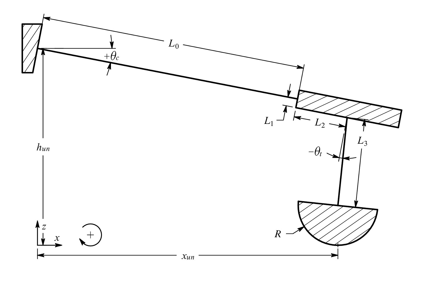
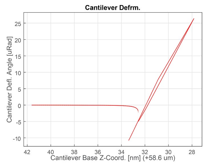
In simulation and experiment, we can see that sample friction affects normal force measurements. Sample friction can and will affect indentation force measurements collected after a "peer-consensus" or "proper" cantilever calibration.

Hidden Lateral Forces

We can see a frictional hysteresis in the experimental and simulated force curves above, but those measurements still don't entirely explain the 17% discrepancy between our quasi-static and oscillatory force curves. A hysteresis is not particularly apparent in the quasi-static sensitivity calibration curve, yet there is still a significant disagreement between the two calibrations.

Let me propose that the observed calibration disagreement is due to "hidden" lateral forces. By "hidden", I mean that the force curve is characteristically ideal: no hysteresis, decent extension-retraction overlap. In other words, the force curve, in its contact region, appears as if it was collected in a perfectly frictionless and elastic environment.

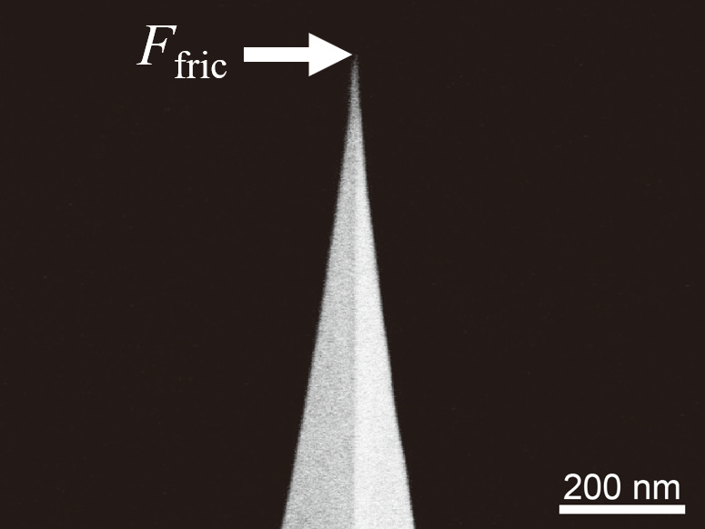
Many AFM cantilevers have long slender tips. What if the long, slender tip was fixed in place, by friction, during the force curve and tip bending (not cantilever bending, rather lateral tip bending) provided the required lateral tip deformation Δx? In this case, there would be no hysteresis because the tip would not slide. To the naked eye, the force curve would appear ideal. However, lateral forces would still be acting at the tip! The lateral forces would create a moment on the cantilever, which would cause the cantilever's deformation to deviate from the ideal quasi-static shape.

This combination of lateral friction and a flexible tip is why our quasi-static and oscillatory sensitivity calibrations do not agree with the predictions of Euler-Bernoulli beam theory.

A schematic of a deformed cantilever with a flexible tip. The angle at the end of the cantilever is reduced due to the moment created by lateral tip-sample forces fixing the tip in place.

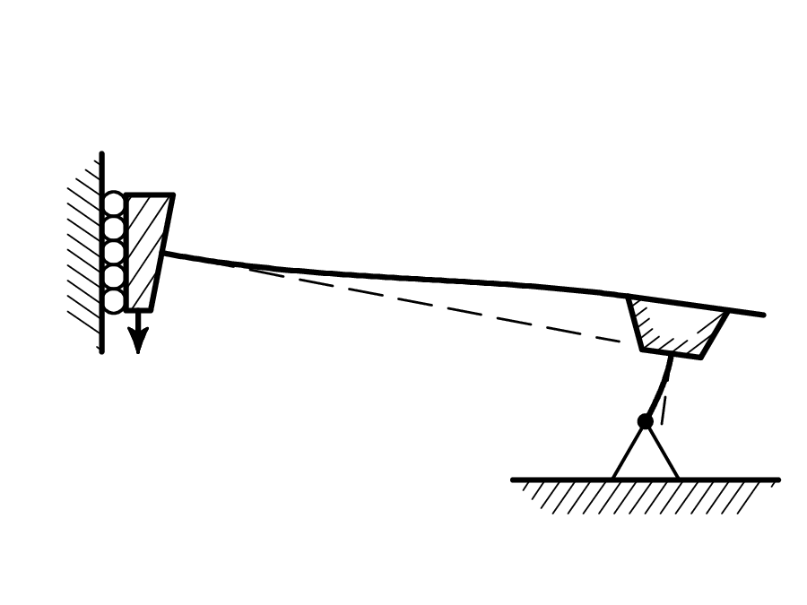
Are tips flexible? Yes. The tips at the end of many commercial cantilevers are often about as flexible as the cantilevers themselves. How do we know? We can approximate a tip's lateral flexibility by building a model of the tip from scanning electron micrographs and computing the tip-beam stiffness.

An SEM image of an Olympus AC Series tip. The quasi-static spring constant of the tip beam is about 10 N/m. Image courtesy Olympus.

Miraculous Tip Levitation

A real force curve (blue) collected from a graphene-coated metal substrate. The vertical axis is the tip-sample force in Newtons. The horizontal axis is tip-sample indentation in meters. This force curve was collected by Matt Robertson. The author reprocessed Matt Robertson's calibrations and measurements and achieved the same non-physical results. The author has added annotations depicting a perfectly rigid (infinitely stiff) force curve, a harder force curve, and a softer force curve to illustrate the non-physicality of this measurement.

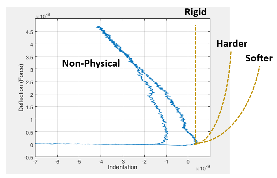
This force curve depicts the indentation of a graphene-coated metal substrate. The cantilever was calibrated using standard, accepted calibration procedures. A quasi-static force curve on sapphire was used for sensitivity calibration. The spring constant was obtained from the cantilever's thermal response.

What is happening here? Why is the cantilever being pushed above the sample surface during indentation? The force curve is clearly non-physical despite following the proper calibration protocols.

Lateral Forces & Graphene AFM Measurements

Why did we obtain the non-physical force curve shown above? Because graphene is nearly frictionless, and sapphire is not. Let me explain.

If we calibrate a cantilever on a sapphire substrate, and if that cantilever has a long, slender tip, and if we press lightly during the sensitivity calibration (as not to damage the tip), then there is a very high likelihood that the tip will remain fixed and bend laterally during the calibration.

The lateral frictional fixing force will reduce the end-of-cantilever angle during calibration. The photodetector will record a smaller signal than what would be expected for the amount of vertical deflection. Therefore, the recorded sensitivity will be less than expected for an ideal deflection of the same cantilever.

When the same cantilever is used to indent the graphene-covered sample, the tip encounters a nearly frictionless surface. With a lack of lateral hindrance, the tip's deformation is more ideal, and the photodetector records a larger signal for the same amount of vertical deflection.

When we apply the low, incorrect sensitivity calibration to the graphene force curves, it will appear that the cantilever deflected upwards quite substantially (and possibly unphysically). This non-physical upward deflection is precisely what we observe in the force curve above.

We are actually lucky if the force curve looks as non-physical as the force curve shown above because that curve clearly indicates a problematic measurement. We could have obtained a graphene force curve with a large but still reasonable modulus showing that we just found a new strongest material.

This erroneous upward deflection is so problematic, especially in hard materials research, because really hard materials don't permit much indentation. A small reduction in measured indentation on a hard material will cause that material to appear much stiffer than it actually is. Unfortunately, as we saw in our example force curve, there is no upper bound to the erroneous stiffening. In other words, AFM measurements of graphene can exhibit infinite, unquantifiable measurement error.

The caveat to this claim is that not all graphene AFM characterizations will be this erroneous. Further, not all AFM measurements will be affected similarly by this phenomenon. Large, stubby tips will respond very differently than long, slender tips.

I will claim, however, that most graphene measurements and most other AFM measurements have unquantifiable error. Why? Because most all commercial AFMs sense cantilever motion using either optical beam deflection (OBD), which measures the cantilever angle, or interferometry, which senses vertical displacement. Both measurements --- OBD and interferometry --- are needed in order to characterize both tip forces --- lateral and normal. If you have OBD without interferometry or vice versa, you are only sensing one of the two degrees of freedom. As we have seen, the unsensed axis can be a source of unquantifiable error.

How do we fix this?

Get a new microscope. Seriously.

Get a microscope that can measure both the angle of the cantilever and its vertical displacement. If you aren't measuring both the angle and vertical displacement of the AFM cantilever, you are missing an entire degree of freedom and therefore have a source of unquantifiable error in your measurements.

I am only aware of one commercially available microscope that can do both measurements: Asylum Research's Vero. (Again, I have no financial ties to Asylum Research. While interviewing at Asylum, I presented this work, which presumably motivated them to develop and market the Vero microscope. Correction: They had just filed a patent for a dual interferometric—optical-beam-deflection AFM, Patent US20220057429A1, and were excited that I had arrived at a similar conclusion.) The Vero combines interferometry and optical beam deflection giving it the ability to simultaneously measure the cantilever angle and its vertical displacement. With both measurements, this microscope can characterize both lateral and normal forces at the tip.

Vindication

For me, the Vero microscope is a bit of a vindication. There were many long, painful years where I fought to develop these ideas only to have them dismissed by a panel of "experts" at my preliminary examination. After that rejection, I reached out to Aleks Labuda at Asylum Research who was kind enough to listen to my presentation and encourage me to continue this work.

Although Asylum Research did not hire me, they still make the best AFM on the market. Aleks is a bit of an AFM and instrument-design wizard who is truly dedicated to the pursuit of truth and excellence in atomic force microscopy.

From Asylum Research's marketing materials, it seems like the Vero's additional measurement axis has eliminated cantilever calibration discrepancies and pleased the folks at NIST. I have no doubt that the Vero microscope will usher in numerous new advances in materials and surface science.

If these calibration and measurement errors have been lurking for so long (20 years or so) in such a widely used technique, what other misconceptions and mismeasurements are still lurking in other corners of science? What will these better measurements help us discover? How will we harness new knowledge and capabilities to accelerate human flourishing?

Postscript

I am not the first to study friction with the atomic force microscope. AFMs have been used to characterize surface friction for some time now. Not mentioned above was the work of Phil Attard, whose work helped guide a lot of these ideas[19][20][21][22]. Aleks Labuda has a number of wonderful works on AFM as well [23][24][25][26].

Post Postscript

What about the factor-of-two error in the formula used for the thermal spring constant? A great number of AFM tips are susceptible to "hidden" lateral force effects due to their long, slender tips. The "hidden" lateral force effects counteract the spring constant error which (1) makes both errors (lateral force & spring constant) much less apparent and (2) makes it more challenging to identify either error since correcting one of the two errors, but not both, makes for worse measurements. Cases like this are why you always check the published math!

Contact

Reach out! Hire me!

Cite this on arXiv. (Coming soon.)

I wrote a MATLAB script for reading files from the AFM.

Behind the work described here lies a lot of rigorous mathematics. I hope to publish this mathematical work over the coming months. For clarity, this post focuses on concepts and discusses only the most necessary mathematics.

Acknowledgments

• The late Scott MacLaren for instilling a sense of wonder in microscopic exploration and, simultaneously, an inquisitive distrust of existing models and explanations.

• Kathy Walsh and Jessica Spear for kindness and support in our shared quest for AFM rigor.

• Aleks Labuda for listening and encouraging me when I needed it most.

• Matt Robertson for his SEM prowess, sharing his red-herring graphene-on-metal AFM measurements, and many valuable discussions. Through no fault of his own, Matt left the academy without a PhD. He put in the time. He's sufficiently bright and hard working. He deserves a PhD.

• Jonathan Bunyan for moral support and a shared desire to pursue truth.

• Adam Mastroianni for brilliantly describing the absurdity and beauty of modern science and pushing myself and others to write. Read his blog: https://www.experimental-history.com/

• Jim Lakowski for invaluable discussions probing the core incentives, objectives, and rewards of the academic-industrial complex.

• My advisor for not kicking me out of UIUC's doctoral program.

• The folks at Quality Beer Co. in Champaign, IL, for providing a warm and supportive community and a constant celebration of midwestern humanity. It takes a village to raise a child and it takes a bar to support a PhD student.

• Special additional thanks to Jim Lakowski and Jonathan Bunyan for reviewing this post.

• Finally, my wife for being a shining light in deepest, darkest depths of doctoral despair.

References

[1] GISAXS, “File:Diamond00.png - GISAXS,” GISAXS Community Website. Accessed: Feb. 19, 2024. [Online]. Available: http://gisaxs.com/index.php/File:Diamond00.png

[2] F. Enam, “A Graphene Primer: From Pencil Lead to Revolution,” A Graphene Primer: From Pencil Lead to Revolution. Accessed: Feb. 19, 2024. [Online]. Available: https://www.aiche.org/sites/default/files/styles/chenected_lead_image/public/images/Chenected/lead/shutterstock114899977.jpg?itok=P-aC7V6C

[3] L. Gross, F. Mohn, N. Moll, P. Liljeroth, and G. Meyer, “The Chemical Structure of a Molecule Resolved by Atomic Force Microscopy,” Science, vol. 325, no. 5944, pp. 1110–1114, Aug. 2009, doi: 10.1126/science.1176210.

[4] Wikipedia, “AFM_tip_with_CO-functionalization.png (722×423),” Non-contact atomic force microscopy. Accessed: Feb. 19, 2024. [Online]. Available: https://upload.wikimedia.org/wikipedia/commons/e/eb/AFM_tip_with_CO-functionalization.png

[5] Asylum Research, “High Resolution DNA,” Oxford Instruments. Accessed: Feb. 19, 2024. [Online]. Available: https://afm.oxinst.com/learning/view/image/high-resolution-dna-1

[6] Asylum Research, “Hard Disk,” Oxford Instruments. Accessed: Feb. 19, 2024. [Online]. Available: https://afm.oxinst.com/learning/view/image/hard-disk

[7] C. Lee, X. Wei, J. W. Kysar, and J. Hone, “Measurement of the Elastic Properties and Intrinsic Strength of Monolayer Graphene,” Science, vol. 321, no. 5887, pp. 385–388, Jul. 2008, doi: 10.1126/science.1157996.

[8] TipsNano, “TGQ1 AFM Calibration Grating Product Description,” TGQ1 AFM Calibration Grating Product Description. Accessed: Feb. 19, 2024. [Online]. Available: https://tipsnano.com/catalog/calibration/tgq1/

[9] R. Proksch, J. Cleveland, and D. Bocek, “Linear variable differential transformers for high precision position measurements,” US7038443B2, May 02, 2006 Accessed: Nov. 27, 2020. [Online]. Available: https://patents.google.com/patent/US7038443B2/en?oq=7%2c038%2c443

[10] R. Proksch, J. Cleveland, and D. Bocek, “Linear variable differential transformers for high precision position measurements,” US7262592B2, Aug. 28, 2007 Accessed: Nov. 27, 2020. [Online]. Available: https://patents.google.com/patent/US7262592B2/en?oq=7262592

[11] Lyons Club, “Adama Innovations,” The Client: Adama Innovation. Accessed: Feb. 19, 2024. [Online]. Available: https://lyons.club/adama-innovations/

[12] J. E. Sader et al., “Spring constant calibration of atomic force microscope cantilevers of arbitrary shape,” Review of Scientific Instruments, vol. 83, no. 10, p. 103705, Oct. 2012, doi: 10.1063/1.4757398.

[13] T. D. B. Jacobs and R. W. Carpick, “Nanoscale wear as a stress-assisted chemical reaction,” Nature Nanotech, vol. 8, no. 2, Art. no. 2, Feb. 2013, doi: 10.1038/nnano.2012.255.

[14] D. A. Walters et al., “Short cantilevers for atomic force microscopy,” Review of Scientific Instruments, vol. 67, no. 10, pp. 3583–3590, Oct. 1996, doi: 10.1063/1.1147177.

[15] B. Cappella and G. Dietler, “Force-distance curves by atomic force microscopy,” Surface Science Reports, vol. 34, no. 1–3, pp. 1–104, Jan. 1999, doi: 10.1016/S0167-5729(99)00003-5.

[16] S. M. Cook, T. E. Schäffer, K. M. Chynoweth, M. Wigton, R. W. Simmonds, and K. M. Lang, “Practical implementation of dynamic methods for measuring atomic force microscope cantilever spring constants,” Nanotechnology, vol. 17, no. 9, p. 2135, Mar. 2006, doi: 10.1088/0957-4484/17/9/010.

[17] R. Proksch, T. E. Schäffer, J. P. Cleveland, R. C. Callahan, and M. B. Viani, “Finite optical spot size and position corrections in thermal spring constant calibration,” Nanotechnology, vol. 15, no. 9, pp. 1344–1350, Aug. 2004, doi: 10.1088/0957-4484/15/9/039.

[18] J. Ralston, I. Larson, M. W. Rutland, A. A. Feiler, and M. Kleijn, “Atomic force microscopy and direct surface force measurements (IUPAC Technical Report),” Pure and Applied Chemistry, vol. 77, no. 12, pp. 2149–2170, Jan. 2005, doi: 10.1351/pac200577122149.

[19] P. Attard, A. Carambassis, and M. W. Rutland, “Dynamic Surface Force Measurement. 2. Friction and the Atomic Force Microscope,” Langmuir, vol. 15, no. 2, pp. 553–563, Jan. 1999, doi: 10.1021/la980848p.

[20] J. Stiernstedt, M. W. Rutland, and P. Attard, “A novel technique for the in situ calibration and measurement of friction with the atomic force microscope,” Review of Scientific Instruments, vol. 76, no. 8, p. 083710, Aug. 2005, doi: 10.1063/1.2006407.

[21] P. Attard, T. Pettersson, and M. W. Rutland, “Thermal calibration of photodiode sensitivity for atomic force microscopy,” Review of Scientific Instruments, vol. 77, no. 11, p. 116110, Nov. 2006, doi: 10.1063/1.2387891.

[22] P. Attard, “Measurement and interpretation of elastic and viscoelastic properties with the atomic force microscope,” J. Phys.: Condens. Matter, vol. 19, no. 47, p. 473201, Nov. 2007, doi: 10.1088/0953-8984/19/47/473201.

[23] A. Labuda _et al._, “Calibration of higher eigenmodes of cantilevers,” _Review of Scientific Instruments_, vol. 87, no. 7, p. 073705, Jul. 2016, doi: [10.1063/1.4955122](https://doi.org/10.1063/1.4955122).

[24] A. Labuda _et al._, “Tapping Mode AFM Imaging in Liquids with blueDrive Photothermal Excitation,” _Microscopy Today_, vol. 26, no. 6, pp. 12–17, Nov. 2018, doi: [10.1017/S1551929518001050](https://doi.org/10.1017/S1551929518001050).

[25] A. Labuda, K. Kobayashi, Y. Miyahara, and P. Grütter, “Retrofitting an atomic force microscope with photothermal excitation for a clean cantilever response in low Q environments,” _Review of Scientific Instruments_, vol. 83, no. 5, p. 053703, May 2012, doi: [10.1063/1.4712286](https://doi.org/10.1063/1.4712286).

[26] A. Labuda, M. Kocuń, W. Meinhold, D. Walters, and R. Proksch, “Generalized Hertz model for bimodal nanomechanical mapping,” _Beilstein J. Nanotechnol._, vol. 7, no. 1, pp. 970–982, Jul. 2016, doi: [10.3762/bjnano.7.89](https://doi.org/10.3762/bjnano.7.89).

[27] An earlier version of this post reported an S0:S1 ratio of 1.07 instead of the correct 1.09. Thank you to Aleks Labuda for noticing this error. Correction applied on 2024-March-14 at 9:50 PM EST.